In this blogpost, we will understand about WAFFLE Chart, their use and how to create static and interactive WAFFLE Charts using Microsoft Excel and Spreadsheets. These charts can be presented using PowerPoint and other presentation tools as well.
Let’s begin with WAFFLE CHARTS
A waffle chart is a data visualization technique that is used to display the distribution of categorical data. It is similar to a square pie chart or a grid-based heatmap. The chart consists of a grid of squares, where each square represents a specific category or data point.
If you are one of those people who are bored with PIE CHARTS, BAR Charts etc, then try WAFFLE CHART. Below is an example of a waffle chart that we have created in Excel. Normally, tt has a total of 100 squares and each square represents one percent of the total value.

Pic : Example of Waffle Chart
Components of a WAFFLE Chart
Now, here are the main components of a WAFFLE Chart which you need to understand before you create it in Excel.
- 100 Cells Grid: You need a square grid of 100 cells (10 X 10).
- Data Point: A data point from where we can take the completion percentage or achievement percentage.
- Data Label: A data label to show the percentage of completion or percentage achievement.
So now it’s time to learn how to create it in Excel. Well, you can use a static or a Dynamic (as per your need). Let’s get started.
Steps to Create a STATIC WAFFLE Chart in Excel
Now, First thing to understand is that – WAFFLE Charts are not the default CHART Type that comes with the Microsoft Excel Chart Recommendations. Hence, you will have to follow the steps below to create –
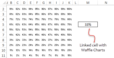
- First of all, you need a grid of 100 cells (10 X 10) and the height and the width of each cell should be the same. The overall grid of cells should be square and that’s the reason it’s called the square pie chart.

- After that, you need to enter values from 1% to 100% in cells starting from the first cell of the last row in the grid. You can use the following formula to insert the percentage from 1% to 100% in the grid (all you need to do is, edit the first cell of the last row, enter this formula and after that copy that formula to the entire grid).
=(COLUMNS($A10:A$10)+10*(ROWS($A10:A$10)-1))/100

- Next, you need a cell for the data point in which you can capture the percentage of completion or achievement. You need to link this cell in the waffle chart further.
- Once you create a data point, next you need to apply the conditional formatting rule on this grid and for this, please follow these simple steps to apply a rule.
-
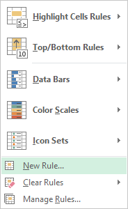
- Select the entire grid and go to → Home Tab → Styles →Conditional Formatting → New Rule.
-
-
-
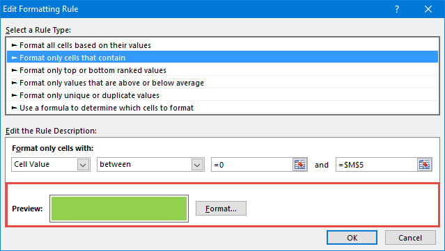
- In the new rule window, select “Format only cells that contain”.
-

-
-
- Now in “format only cells with” specify the values 0 as a minimum and $M$4 as maximum values.
- This rule will apply the conditional formatting to the cells which have the value between this value range.
-

-
-
- Click on the format button to specify a format to apply.
- Make sure to apply the same color for font and cell color to hide fonts when conditional will apply.
-
- From here, you need to apply a final formatting touch and for this select the grid and do the following:
-
- Change font color to white.
- Apply a white border to cells in the grid.
- Apply a solid outer border to the grid with black color.
-
- After doing this you will get a waffle chart that is linked to a cell and when you change data in that cell the chart will get automatically updated.

- Now, you need to create a label for the chart and you need to insert a simple text box and connect it to the cell. Follow the below steps for this.
-
- Insert a text box in your worksheet from Go to → Insert Tab → Text → TextBox.
- Now, select the text box and click inside the formula bar.
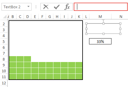
- Enter cell reference of data point cell and press enter.
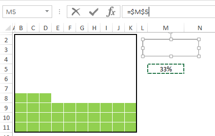
- Increase the size of the font and place the text box on your chart.
-

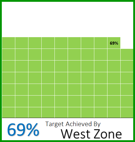
Now your WAFFLE chart is ready and you can use it anywhere, but, We want to add something more and we are sure you’ll like it. In the below chart, apart from the main label, we have a small label at the last square of the grid which can help the viewer instantly identify the chart’s value.
To add this label we need to follow below steps:
Now, in order to put the label, follow the steps below;
- First of all, select the entire chart grid and go to the Highlight Cell Rules ➜ Equals.

- Now in the equals to the dialog box, in “Format cells that EQUALS to” select the cell where we have our percentage value.

- After that, open “Custom Formatting” and go to the “Font” tab.

- From here in the font tab, select the “White” font color and click OK.

The moment you click OK it’ll add a small label (which is the cell value) in the last square.

Congratulations! your first Excel waffle chart is ready.
Steps to Create an Interactive WAFFLE Chart
From the above steps, you know how to create a WAFFLE chart. Now, let’s try to make it an interactive one.
In the interactive one, you will have control on how the data shows with each feedback from the user. We will use BUTTONs to change the data and make WAFFLE Chart more interactive.

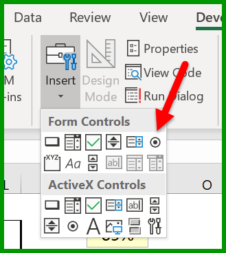
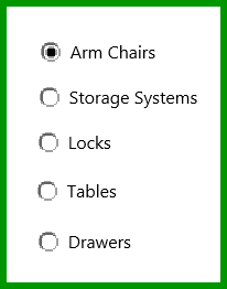
- First of all, you need to insert five option buttons into the worksheet and for this go to the DEVELOPER Tab ➜ Insert Option Buttons.
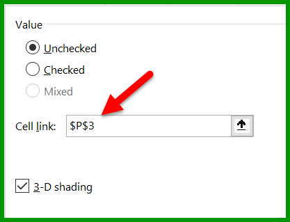
- After that, you need to connect those option buttons to a cell. So when you select a button that cell can have a number which we can use to extract data from the main table.
- For this, select all the option buttons and right-click and then select “Format Control” (You can also group all the option buttons by using the GROUP option).
- Next, you need to name all the five option buttons as per the product names you have. Simply right-click and edit text.
- Now the next thing is to create a formula and insert it into the achievement cell so that when you select an option button it returns the value for that particular product.
- So that formula we need here would be like =INDEX(R6:R10,P3)
- Enter the above formulas in the achievement cell. In this formula, R6:R10 is the range where you have achievement values and P3 is the cell that is connected with the option buttons.

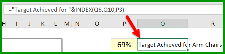
- There’s one more thing which we need to do and that’s creating a dynamic label for the chart (at this point, we have a data label which is connected to the achievement cell but we need to make it dynamic).
- For this, we need to enter the below formula in the cell next to the achievement cell =”Target Achieved for “&INDEX(Q6:Q10,P3)
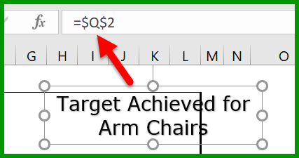
- After that, insert a simple text box that you need to connect with the cell where you just added the above formula and for this select that text box and click on the formula bar and type the address of the cell where you have the formula.
Now you have an INTERACTIVE CHART in your worksheet which you can use and control with the option buttons.

Conclusion
To Sum up, we have understood the basics and some advanced level features in Microsoft Excel to create WAFFLE Charts. Now, Waffle charts are useful when you want to display the relative proportion or distribution of categorical data in an easily understandable and visually appealing manner.
They are particularly effective when the number of categories is small, as larger numbers of categories can result in a crowded and less interpretable chart.